Name Range in Excel

What is a Name Range ?

Name Range in Excel, a name  to any cell, a range of cell, selection of a area, after naming the cell or area or a range of cells we only need to remember the cell or area reference by its name not from the cell or range reference.

Benefits of Name Range

1.   After naming the cell or range or selected area we do not need to remember its cell address or      

      reference.

2.   After naming the cell or range or selected area, now it will becomes very easy to put name in    

      formula and function.

3.   Name Range data always remain constant and does not change its cell references.

Below are some methods of Name Range Data

  1.   Using the Name Box
  2.   Using the Create from Selection Command
  3.   Using the Define Name command

Below we will discuss the the each of above mentioned heading of Name Range in Excel

1. Using Name Box

In Excel, we can create a name range by selecting a cell or a range of cell and typing a appropriate name in the "name box" field.  See the image below

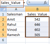
In the below given image we have data set, in column 1st we have "Salesman" and 2nd column we have "Sales figure" of "Sales_value". So we will name range in this data that from range "B2:B5" we give a name as "Sales_Value" and type this name in the field of "name box"

Image 01

See below image :-

   

Image 02

In above image we can see data range "A2:A5", so according to name range rule we can give a name to this entire range by selecting the whole range area and typing the name in the name box field "Student".

So whenever we need to write any formula, then we do not need to give the entire range, then just name range require, like the whole area = "Student"

We want to sum sales value of all the Student, so the formula will be :-

=Sum(Sales_Value) or =Sum(B2:B5) bot are same.

Without giving a sales range, we mention directly "Sales_Value" instead of "B2:B5" and get the same result.

Image 03

2.   Using Create from Selection Command

This is the second method of creating name range. If we have a data set then for creating a name is simple process by selecting the data 

First we need to select the data range and then 

Image 04

go to formula tab, and click  on "Create from Selection"  or short cut key is "CTR+SHIFT+F3" see below image 

Image 05

Once the "Click" the following image will appear :-

Image 06

In this image we can see that there are two image 1st image is "data range" and 2nd image is "how to create name range" image. in this 2 image "Top row" and "Left column" both are checked it is suggesting us that if we press simply "OK" then it will create a name range. All the heading of all "Row" and "Column" will be names of their respective rows or columns."Top row" heading "Salesman", "East", "West" etc. and "Left column" heading will be "Amit", "Rahul" etc. See below image :- 

Image 07

When we select a rows from "B3:E3" it gives a name of this range as "Rahul" as "Left heading" and in second image when we select "C2:C5" it gives the name "West" as the "Top row" heading

So this is another example of  Name Range" of cell or range of cells.

 3.   Using Define Name command

There is another method for creating a name range in  Excel. We have a set of data as given in the following image :-

Image 08

For creating the name range with the help of "Define Name" method we have to go "Formula Tab " and click on "Define Name" drop down and click on "Define Name"

 

Image 09

We will get the following image

Image 10

From starting, see "New Name" name is "West" and then scope "Workbook" or "Sheet no." and at the end "Refers to:" "C2:C5" and simply press enter. And the name range is set for range "C2:C5" is "West"

In the field of  "New Name" instead of West we can put any name according to out need but there are some condition for putting a name and the condition are as follows:-

   

•  Name should not contain more than 255 character and begin with a letter, an underscore( _ ), or backslash(\) and should not contain any space

• Name  should not conflict with cell reference like "A1" or "B21"  or so on.

• Single letters will be OK for name like "A", "B", "F", etc), but "R", and "C" are not allowed they are reserved and "R=Row" and "C=Column"

Edit a Name Range

Some time if we have to edit our name range then what to do?

So in this case we need directly go to "Name Manager", see image below :-

Image11

and simply click on it we will get the following pictures :-

With help of above image we can easily modify or edit our name range.

Delete a Name Range

Now if we want to delete a name range  in excel simply go to "Name Manager"  and click we will get the following image and just click delete on it, the name range will be deleted. See below :-

So in this tutorial we learned about name range in excel. Name range has many more uses if we will go into deep of name range, we will learn more about it.

Thanking you.

Regards

NarendrasExceltips.blogspot.com

Excel Data Validation

Excel Data Validation is a option in excel by which we  can restrict the operater by typing the false entry in the Excel sheet, it has some criteria for user and from this criteria or condition the user can not enter the wrong input.

We will understand this by following example:-

Go to Data Tab -->

Image 01

In this this image we can see that in the Data Tab --> Data Validation and when we click on Data Validation following image will appear

Image 02

In this 2nd image, there are three table ---> "Settings", "Input Message", "Error Alert" and then Validation criteria "Allow" :- Any Value

When we select a area in excel and apply this condition in data validation, this criteria accepts all the numbers or text, it does not have any restriction to the field. But when this feature will  restrict us to put incorrect data, we will learn in further in this  blog.

Now come to the second image :-

image 03

This is the all list of data validation :-

"Whole number", "Decimal", "List", "Date", "Time", "Text length", "Custom".

We  will discuss all of the above given option one by one.

"Input Message " is the second tab in the Data Validation box and the third one is "Error Alert"

Input Message box in Data Validation

Image 04

"Input Message" box display the message about the cell or area containing the validation about, like in the above image we can see that we  have a message like in "Title = => Serial No." and in the "Input message" box "Only put serial no. 1 to 10" and same we can see above in the excel coloured area, when we put our cursor into cell "C1" it displays the message as we put in the "Input message" box.

Error Alert box in Data Validation

See the image below :-

Image 05

Now in this Data Validation "Error Alert" message box,  we notice that we have checked the check box "Show error alert after invalid data is entered" if we do not check this check box then the message will not be displays.

Now come to "Style" and the option are "Stop", "Warning" and " Information" all the option are available for we that in which option we want to see the message from these three option.

Then "Title" is that what title we want to give that error message, we have put Wrong Input.

Then "Error Message" what message will pop up when someone will put wrong data in the validation field.

See the  below image :-

Image 06

We put "11" in the coloured field that field has validation and the message is showing that "Wrong Input" as the error title and message is "Please enter the no. between 1 to 10 only" this coloured area has validation to put data only from 1 to 10 not beyond this.

Criteria Examples of Data Validation

Any Value Data Validation

If we select this option in data validation that means we can put any data into the data validation field whether a numeric or a text one.

Whole Number Data Validation

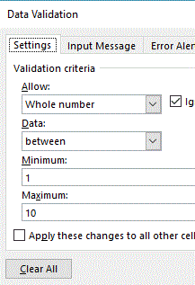
Now come to second option Whole number, if we choose this option that means we can specify the maximum and minimum range in the validation area, see the image below :-

Image 07

We have set the limit between minimum "1"  and  maximum "10" the data validation field will accept the data with-in this range only not apart from that.

Decimal Data Validation

In this image we can see that we have set the data validation value  from 100 to 125 and this has a additional feature that it can accept the decimal figure also, like in the below image we can see "100.253" and "124.362" but not greater than "125". It accept the value in decimal also.

Image 08

List Data Validation

Now move forward to another option and it is "List" option in data validation. See the image below 

Image 09

In this image we can see that in cell "A1 to A3" we have put some name and now  the cursor position in cell "B1". In the "List" option in data validation, select "list" from allow field and type all the names in the "Source" field or drag the name range from "A1:A3", result would be same from both option and press "OK" then go to cell "B1" the following image will appear.

The drop down menu have been created by simple pressing "OK" button.

Image10

In the above image we can see that when we click on cell "B1" then a drop down menu list open with containing all the list details of from "A1 to A3".

Date Data Validation

In the below image the selected area has a data validation for the "date range". From start date contain the date range of cell "A1" and end date range contains the date of cell "B1".

Image 11

If any other date will be entered in the selected validated area the date will not be accepted by excel.

Time Data Validation

In the below image we have put the time range  in start time and end time and the selected area will not accept any time range apart from this time range.

Image 12

Text Length Data Validation

Text length validation option gives a condition that we can put the  text into a validation area, that we can only put the data according to the condition as shows in the below image.

Image 13

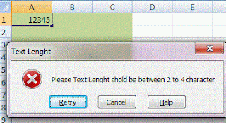
And if we try to write something beyond our validation condition  then it does not allow us to do that by showing below error message ,

Image 14

Custom Data Validation

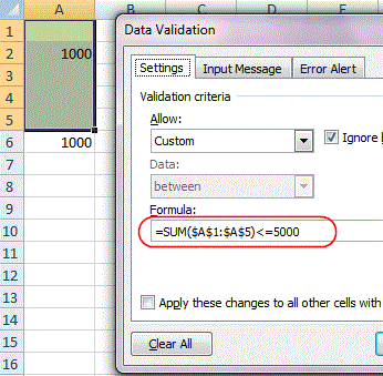
Custom data validation is the validation when we put our own condition in the formula point and get the result as appear in the below image :-

Image 15

And if we enter the value beyond  criteria then it shows the below message :-

Image 16

In this Custom Data Validation option we can create more formula's according to our need. 

Circle Invalid Data

If we have a data range and this data range contain a data validation of any given range as in the following image :- 

Image 17

In the above image we can see that we have given a range from 100 to 150, so the data range will accept the data from this criteria only but if there is any data beyond this range it will circle the cell, which is containing the the wrong value.

How to do that, just see below instruction and image :-

Excel Data - ->Data Validation --> Circle Invalid Data 

Image 18

and once you click on the "Circle Invalid Data" then the following result will come out from the selected data range which is containing the data validation.

Image 19

In this image we can see that which figure is beyond our data validation limit i.e. 100 to 150, the "Circle Invalid Data" option put a circle around that figure and again if we want to remove the circle then we have to follow this command. 

Go to Data -- ----  Data Validation ---- Clear Validation Circles and click on it.

Image 20

Once you click on the button "Circle Validation Circles" we will get the following image :-

Image 21

All the  red circles have been removed.

How to Remove Data Validation

Now we have learned all the option in data validation and now we will learn about how to remove data validation. Now simply follow the step 

Click Data ---- Data Validation ---- Click on Data Validation button and then click "Clear All" button, appearing below in the given image and then "OK" 

Image 22

All the data validation have been removed from the selected area and we can work on Excel as normally.

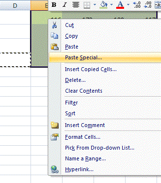
There is one more way to remove data validation from the given range. Simply go to a blank cell which does not contain any validation and copy it the go to the validation area and select all the validated area and right click as mentioned in the below image and clikc on  paste special.

Image 23

Once you clik on paste special you will get the following image :-

Click on the "Validation" radio button and simply press "OK" and we are done.

This is very easy way to remove data validation from easy step.

Thanks and Regards

NarendrasExcelTips.blogspot.com