How to Change Font Color in Excel VBA

In this blog post, you will learn about how to change the font color in Excel VBA.

Suppose that we have some text dataset from range “A1: B6”, and want to change the color of this.

See below text dataset image:-

Here we have two methods to change the “Font” color of a dataset.

First Method: Font.Color

Second Method: Font.ColorIndex

See below both the method explained one by one.

First Method: Font.Color 

This is our first method to change the “Font” color of our dataset.

First of all, go to the Developer tab in Excel.

Once the “Visual Basic” window opens then Go to “Insert” and open a new “Module”.

The new “Module” opens.

Then write the following code:-

Because here, in the above image our dataset exists between range “A1: B6”.

So our VBA code will be:-

“Range ("A1: B6").Font. Color = vbRed” and then press “F8”. See the font color has been changed.

In this method, we have 8 standard colors to change the font color of our dataset.

See below all 8 standard colors, write these codes in Excel Visual Basic Editor and run it by pressing “F8” (step by step).

See the text color changed one by one.

Second Method: Font.ColorIndex

In this method, we have more options to change the “Font” color of our dataset.

Now again, we will follow the same way to enter into the visual basic editor.

In the previous method, we can change the font with 8 standard colors only.

In this method (Font.ColorIndex), every single number from 1 to 56, is assigned a particular color.

See in the below image, here are some random number applied.

You can apply for the number up to 56.

So, these are the two methods to change the “Font” color of a text or a text dataset.

I hope you find this useful.

Please feel free to put our comments.

Regards

How to Change the Background Color in Excel VBA

3 Easiest Way to Copy and Paste Data in Excel VBA

How to Change the Background Color in Excel VBA

In this tutorial, you will learn about how to color the background of a cell or range.

There are two easiest methods to change the background color of a cell in Excel VBA.

1. Interior.Color
2. Interior.ColorIndex

First Method: - Interior.Color

In this method, we will learn how to apply the background color.

Suppose that you want to color the background of range (“A1: B6”) in our Excel sheet.

See the image below:-

Now, we will write the VBA code to color the background of the range (“A1: B6”).

Go to the developer tab à Visual Basic à on visual basic editor window --> Go to Insert and click on “Module”.

Once the module is opened,

Write the following code in the inserted module:-

In the above image, we have applied the “Green” color by VBA coding.

The same way we can apply 8 standard colors by VBA coding.

These 8 standard colors are as follows:-

1.     Black (vbBlack)
2.     White (vbWhite)
3.     Blue (vbBlue)
4.     Red (vbRed)
5.     Pink (vbYellow)
6.     Green (vbGreen)
7.     Cyan vb(Cyan)
8.     Magenta (vbMagenta)

See all these 8 standard color codes in VBA:-

Method 2:- Interior.ColorIndex

This is the second method to color the background of a cell or range. In the previous method, we applied the 8 standard colors in the given range.

But in this method, we can apply the color from 1 to 56.

Every single digit has a specific color from 1 to 56, but after this number, this method does not work.

Now, we write our code to apply the color in a cell or range, see below:-

“Range(“A1:B6”).interior.ColorIndex=1, and the same way we can write our code from 1 to 56 numbers.

For example, see below:-

These are the two methods to color the background in Excel VBA.

I hope you find it useful.

Thanks

3 Easiest Way to Copy and Paste Data in Excel VBA

How to Change Font Color in Excel VBA

3 Easiest Way to Copy and Paste Data in Excel VBA

In this blog post, we are going to learn 3 best and easiest way to copy and paste data from one place to another within the same worksheet.

Below are these 3 methods:-

1. Range.copy method
2. Destination = Source Method
3. Paste Special Method

First Method:

Range.Copy

Suppose that we have a dataset from Column “A1: A10” and we need to copy and paste this whole data into another location, such as in Column “D1: D10”.

Now we will apply the VBA code to copy and paste the above dataset in the desired location.

Please see below:-

First type “Range (“A1: A10”).copy and then press “Space bar”, this will ask the destination location. Then write code such as “Destination: = desired location Range”.

Here “C1: C10” is the desired range where we paste our dataset.

Second Method: 

Destination = Source Range

This is the second method, in this method we follow the rule of Excel VBA such as:-

Destination = Source Range

“Range where we want to paste our data" = "our source data range, which we want to copy”.

Destination: - This is the destination area where we want to paste our dataset within the worksheet.

Source Range: - Our source data, which we want to copy and paste it in another place.

Please see below the simple VBA coding:-

Third Method:- 

Paste Special

This is our third method to copy and paste dataset in Excel VBA.

Step 1. – In this method, first we will write down our code to copy data from source data.

Step 2- Then, write the code to paste the dataset into the destination field.

Step3:- Once the dataset is copied the “CutCopyMode” appears around whole the dataset. To remove this “CutCopyMode” we need to apply the code as shown in the image below.

“Application.CutCopyMode = False”.

 These are the three best and easiest VBA Codes to copy and paste the data from one to another place, within the same worksheet.

I hope you find this tutorial helpful.

Please feel free to put your comments and suggestion on this post.

Thanks and Regards

Narendra


How to Change the Background Color in Excel VBA

How to Change Font Color in Excel VBA

How to Set a Password in Excel File

Today in this tutorial we will learn about protecting our Excel file by putting  a password in it. by doing this will keep our documents safe and secure.


"Caution: If you lose or forget the password, it cannot be recovered. It advisable to keep a list of passwords and their corresponding workbook ans sheet name in a safe place (Remember that passwords are case-sensitive.)"


There are two ways to put  password in the documents :-

1. Password to Open

2. Password to Modify (Open with Read Only)

We will learn about each of these topic one by one.

1. Password to Open

When we put password in Excel by this way then nobody can open the password protected file without putting correct password in it. With the help following image, we will learn how to do this.

Suppose we have a Excel data file and we want to make this file as password protected.  So to do that we have to follow the simple step as given below.

Go to  Office button in office 2007 and click and then click on "Save As"

Image 01

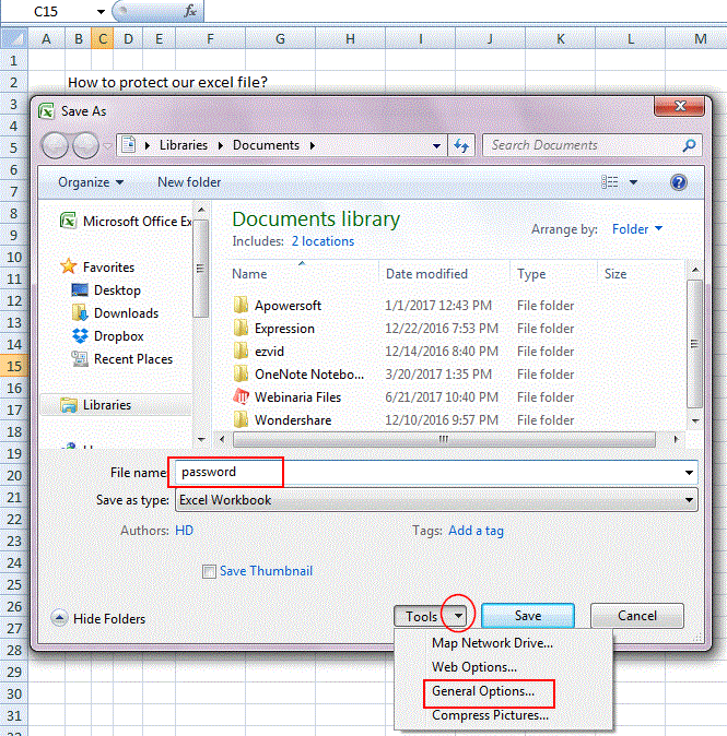
Once we click on "Save As" button, we will get the following image of saving the document.

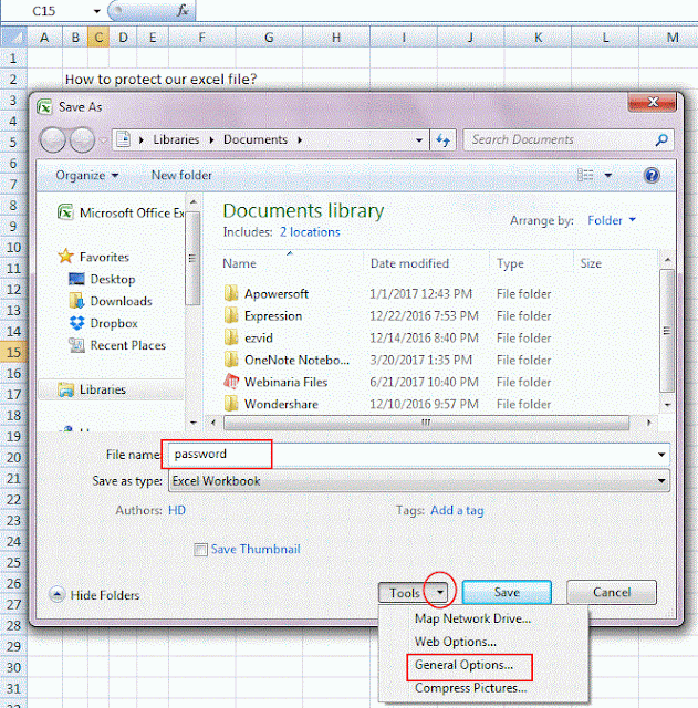
Image 02

We have put the name of the file as "password" and then click on the tools button given below red circled, click on the drop down and we will get the  four other options.  

Click on the "General Options" button and we will get the following image.

Image 03

1. Password to Open

We use this option when we want that nobody can even open our document and can't see it.

Simply put the password in the 1st "Password to Open" and press "Enter".

  

Image 04

We will get the below given image for asking us to put password again. Remember that we do not need to put password in the "Image 03" on both the field i.e. 1 and 2.  1 is for different use and 2 is for different use.

So after pressing Enter, enter the password again in the given field and simply "OK" and our document is save.

Image 05

Now we need to open the document but I want to remind one thing that in the above "Image 04" there is a "Read-only recommended" option is available, so when we check this option the document will open in the two form. 1st is in the "read-only "mode, in this mode we can not modify the data and 2nd option is to open in the normal mode.

When we will open the document, we will get following option to put the password.

Image 06

  When we will put the correct password in it, it will ask another option to us to open it on "Read-Only" mode or "Normal" mode.

To open this document in the form of "Read-Only" mode, it means, we do not need to change anything in this document else open it into normal mode and can change the data.

Image 07

We will open the document in the both of the form "Yes" and "No" . First press  "Yes" and see what happens. 

Below image when we open the document in the "Yes" form i.e. "read-only" form and want to edit some data, like typing "Hello" and save it. It will not save our data and pop up the following error. The document is showing as "read-only", see top with the file name[Read-Only] appears.

Image 08

Now we will open this document in the form of "No" and see what happens :-

Image 09

The file is simply opening in the normal mode and can editing the data also.

2. Password to Modify (Open with Read Only)

Now come to the second option of the protecting the document with "Read-Only" mode.

Follow the instruction as we follow in the above method and reach to "Tools" option and see the below image.

Now in this time put the password in the second filed i.e. "Password to modify" and  Enter

Image 10

After pressing the enter we will get the following image and again put the same password in the given field. and press enter and save the document. Now our file is password protected file and no one can see this document but can see as "read-only" mode.

Image 11

Save the document and open it.  See below image  :-

Image 12

Now we have save  this document in the of "Read-Only" mode so when somebody open this document it will open in the "Read-Only" mode and anybody can open and see the data but can not edit or save the data without having the password.

How to remove password 

Now we will learn to how to remove the password from the password protected file.

We will follow the same way as we entered the password the same way to remove the password from the file.

Go to File Office Button Click and Click Save as button and go to tools and click on drop down and click on General Option and we will get the following image 

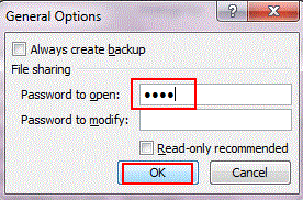
Image10

And now delete the password from the field and save the document, the password has been remove from the document.

Now today we learned, how to make our document as password protected and how to make the secure our data.

We will learn something new in the next tutorial.

Thanks and regards

NarendrasExcelTips.Blogspot.com

Name Range in Excel

What is a Name Range ?

Name Range in Excel, a name  to any cell, a range of cell, selection of a area, after naming the cell or area or a range of cells we only need to remember the cell or area reference by its name not from the cell or range reference.

Benefits of Name Range

1.   After naming the cell or range or selected area we do not need to remember its cell address or      

      reference.

2.   After naming the cell or range or selected area, now it will becomes very easy to put name in    

      formula and function.

3.   Name Range data always remain constant and does not change its cell references.

Below are some methods of Name Range Data

  1.   Using the Name Box
  2.   Using the Create from Selection Command
  3.   Using the Define Name command

Below we will discuss the the each of above mentioned heading of Name Range in Excel

1. Using Name Box

In Excel, we can create a name range by selecting a cell or a range of cell and typing a appropriate name in the "name box" field.  See the image below

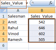
In the below given image we have data set, in column 1st we have "Salesman" and 2nd column we have "Sales figure" of "Sales_value". So we will name range in this data that from range "B2:B5" we give a name as "Sales_Value" and type this name in the field of "name box"

Image 01

See below image :-

   

Image 02

In above image we can see data range "A2:A5", so according to name range rule we can give a name to this entire range by selecting the whole range area and typing the name in the name box field "Student".

So whenever we need to write any formula, then we do not need to give the entire range, then just name range require, like the whole area = "Student"

We want to sum sales value of all the Student, so the formula will be :-

=Sum(Sales_Value) or =Sum(B2:B5) bot are same.

Without giving a sales range, we mention directly "Sales_Value" instead of "B2:B5" and get the same result.

Image 03

2.   Using Create from Selection Command

This is the second method of creating name range. If we have a data set then for creating a name is simple process by selecting the data 

First we need to select the data range and then 

Image 04

go to formula tab, and click  on "Create from Selection"  or short cut key is "CTR+SHIFT+F3" see below image 

Image 05

Once the "Click" the following image will appear :-

Image 06

In this image we can see that there are two image 1st image is "data range" and 2nd image is "how to create name range" image. in this 2 image "Top row" and "Left column" both are checked it is suggesting us that if we press simply "OK" then it will create a name range. All the heading of all "Row" and "Column" will be names of their respective rows or columns."Top row" heading "Salesman", "East", "West" etc. and "Left column" heading will be "Amit", "Rahul" etc. See below image :- 

Image 07

When we select a rows from "B3:E3" it gives a name of this range as "Rahul" as "Left heading" and in second image when we select "C2:C5" it gives the name "West" as the "Top row" heading

So this is another example of  Name Range" of cell or range of cells.

 3.   Using Define Name command

There is another method for creating a name range in  Excel. We have a set of data as given in the following image :-

Image 08

For creating the name range with the help of "Define Name" method we have to go "Formula Tab " and click on "Define Name" drop down and click on "Define Name"

 

Image 09

We will get the following image

Image 10

From starting, see "New Name" name is "West" and then scope "Workbook" or "Sheet no." and at the end "Refers to:" "C2:C5" and simply press enter. And the name range is set for range "C2:C5" is "West"

In the field of  "New Name" instead of West we can put any name according to out need but there are some condition for putting a name and the condition are as follows:-

   

•  Name should not contain more than 255 character and begin with a letter, an underscore( _ ), or backslash(\) and should not contain any space

• Name  should not conflict with cell reference like "A1" or "B21"  or so on.

• Single letters will be OK for name like "A", "B", "F", etc), but "R", and "C" are not allowed they are reserved and "R=Row" and "C=Column"

Edit a Name Range

Some time if we have to edit our name range then what to do?

So in this case we need directly go to "Name Manager", see image below :-

Image11

and simply click on it we will get the following pictures :-

With help of above image we can easily modify or edit our name range.

Delete a Name Range

Now if we want to delete a name range  in excel simply go to "Name Manager"  and click we will get the following image and just click delete on it, the name range will be deleted. See below :-

So in this tutorial we learned about name range in excel. Name range has many more uses if we will go into deep of name range, we will learn more about it.

Thanking you.

Regards

NarendrasExceltips.blogspot.com