Grouping Data In Pivot Table

    
"Grouping Pivot Table" comes in rescue when we have a huge data on daily basis and we have to compile the data so it is not possible to make a pivot table on daily basis data then we have a option of Grouping Pivot Table.

What Grouping Pivot Table option does, it converts days wise data  into "Months", "Weeks", and "Years" according to our need.

So this is the main reason of using  "Grouping Pivot Table" option.

Like in the below given image we have the data for each single day,  so if we have a huge data around 10 to 15 thousands of rows by date wise. So Grouping is the only option to make a Pivot Table reports. 

The below given pivot table is without “Grouping Pivot Table” option and we can see that it is too long and difficult to calculate data accosting to individual date wise but when we calculate the data by the Date which falls on the same month, like the data of Jan, Feb, Mar, etc. then it will be very easy to create a Pivot Table.

So for grouping the data simply right click on the pivot tale on the date column and then select Grouping option it looks like as below given image

And when we click on Group option it looks like the below given image

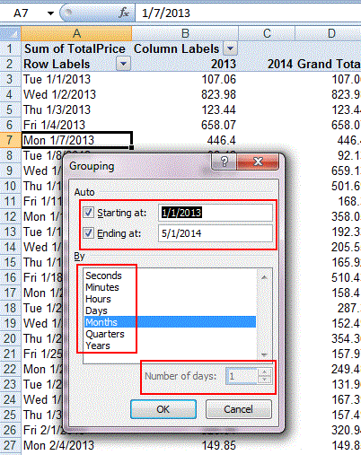
1st box you can see that “Starting at” and “Ending at” you can give the start date by your choice and it will generate the Pivot Table according the data select, it will only given range between the selected period.

2^nd box is the main box you can convert your data by “Years”, “Quarters”, “Months”, “Days”, “Hours”, and so on as its mentioned on the list.

3^rd box represents that,” if you want weekly status then 3^rd box comes in rescue like you can increase that “Number of days:” by 7 and it will provide the data according to weekly basis.

Now if you click on month  and press “OK” button the following Pivot Table will appear.

Now all the date have been convert into “Month”, this option will cumulate all the date wise data in a month and all the month names are appearing  in the pivot table with the cumulative data with column “2013” and “2014” respectively and the Grand total as well.

This is the month wise data and by the Group Pivot table we can generate the data by “Year wise” also and “By the Month and Year wise also”. Like in this below mention image the data will be according to “Year and Month”

Grouping Dates by Week

In the below given image we can generate the report by weekly basis also by selecting the “Days” and increasing the “Number of days: 7” and then click ok

When we click “Ok” button then we will have the  below given image

So this tutorial was completely dedicated for Grouping in Pivot Table and there are another       

more feature in Pivot table, we will discussed in further tutorials.

Narendra

Pivot Tables

Pivot Tables are one of the most useful tool in excel, and most excel experts says that

this tool is the magic tool for quickly prepare report from huge data  set within a few   second.  

This is so useful and powerful tool that within a few second we can make report according to our need. We will learn here in details about Pivot Table beginning part. Below are the screenshot of the data set from which we will prepare the report.

               

Vlookup formula for multiple columns

  Hi friends,

            Today we learn about how Vlookup can retrieve the value of  multiple columns from a single 

formula.

Lets learn the matter with the following example :

We have a table above with Name in column A and East, West, North, South in the row 1 field and 

table has some random data within the table range from A1:E7.

Now to understand the example in a better way we have to draw a second table with no data, is 

mentioned below:

Now we have a blank table and this table has no data and with the help of given data in Table1 there 

is one way we are familiar with i.e. simply type formula =VLOOKUP(H1,A1:E7,2,FALSE) but  

this formula is basic formula and to look for each record we have to type the formula every single 

time, but today we will discuss about a single formula to drag all the cell result.

So here is another table to understand it in better way.

I have typed the formula above and described it below

1.       Lookup_Value      :  We are looking the value of H1 in column I1 from Table1

1.       Table_array          :  We will the find the value of this cell from  table range $A$1:$E$7 (Table1)

1.       Col_Index_num   :  Now this is the main field column, we will look for the value of each column

    

                                               by typing the vlookup  formula in each column, but by the help of vlookup columns

                                           

                                               formula we do not need to type the vlookup formula each time, we will                                                  

                                       understand it from above mentioned example(Table3).

      

        False                   :  And the last argument is True/False(Approximate/Exactly)

In the above mentioned example you are watching that there are $ sign in the formula, this $ has a 

important role in formula writing in Excel and we can put this $ by pressing F4 key repeatedly to get

 the result accordingly. This $ sign fixing a row or column i.e. $H1 (H: Column, 1: Row), 

$H1  column  (H) will be freeze and will not change but row 1will change whenever we will drag it 

right  or down.

So if you will exactly type the above formula in the table and press Enter, it will retrieve all data from  

Table1, all fields will get their data automatically.

I  will give a separate post for Absolute Cell Reference  later 

Now focus on third arguments i.e. Col_index_num COLUMNS($B1:B1)+1

Here is the detailed description $B1:B1 represents the same column but  when  you drag it first $B 

will be  remain same and second B will be change to C, D, E, F and so on and after closing the 

bracket type +1 and it will automatically look for the next column, you can see by deleting the +1 

from the formula and see then what happened. 

So friends , soon I will be back with another useful post 

goodbye for now

Narendra

The Vlookup Guide

    
      Today we will discussed about the most useful topic of advance excel, so for us it is necessary to know that how to use this function and why this function is so much useful.

First we will understand that what is vlookup and why this is so important so first we will put a little 

look what is vlookup.

VLOOKUP, V stands for "vertical" which mean use VLOOKUP to lookup values in table that's 

arranged vertically. And the same for Hlookup stands for “Horizontal” but we will discuss that in later.

                         VLOOKUP (Lookup_value, table_array, col_index, [range_lookup])
                                                    (1)                     (2)             (3)                   (4)

(1)    Lookup_value          The value to look for in the first column of a table

(2)    table_array               The table from which to retrieve a value.

(3)    col_index_num       The column in the table from which to retrieve a value.

(4)    range_lookup           [optional] TRUE = approximate match (default). FALSE = exact match.

Here is the example:-

Here we will discuss about one by one but for the clarity we need one table to understand the picture clearly.

Here in this above image we can see that row no 3 is highlighted, suppose that  we have only cell value “George” in cell A3 and we have to look for the cost of “George”or we need to find the value of “Profit” of “George” so in this case we can use vlookup and after using vlookup we can get the value easily. How to find the value of “George”  in the column of “Cost” or “Profit”, see how it happens :- 

Simply type =Vlookup(1,2,3,4)

                    =Vlookup (lookup-value{ we are looking for},table-array{total table area from A1 to D9},col-index{in which column we the value is exist},[range-lookup]{iether we want exact value or near about}               

Now we need to put the value in the above format

       =Vlookup(A13,A1:D9,3,False)

      A13      =we are looking for “George” value in cost column so “George” is located in cell A13.

      A1:D9  =total table area, we can easily seen that total  data is from cell A1:D9

     

      3          = 3 is the column no. where my value is located

True/False =    and last argument is True/False which means either we want the value exactly or near about will do.      

After putting these value into the formula and press enter, you will get the result that “George” gave “7412” value in column 3 and if in the formula we will change column no. “4” instead of “3” you will get the result  from 4^th  column i.e. = 12025 the value of “George” is located in column no. “4“

Limitations of Vlookup

Vlookup has some limitation and in the following example we will discuss about it.

1.        Vlookup will always look for the data from extreme left to right, not from mid to right , in the below given image  vlookup will find the data from Column A to Column D not form Column B to Column C  or Column D. 

We can understand it from below given example :-

 We have cut a piece form above image to understand this better way and in this below given screenshot we can  see that column (H) and column (I) are blank but we can find the value for both the places.

By the vlookup formula if we want to look for the value for H2 and I2 the formula would be

=Vlookup(F2,Table array would be (A1 to D9), column no would be 3 or 4, and last step  is True/False)

True stand for = Match nearest value

False stand for = Match exact value

I want to say from this example we cannot find the result by putting the below given example

=Vlookup(G2,Table array would be (A1 to D9), column no would be 3 or 4, and last step  is True/False)

=Vlookup(G2, A1 : D9, 3 or 4, False)

If we are applying this formula so we have to take notice that when we will look for G2 so the table array would be B2:D9 not by A1:D9 if we follow this the result will be come out because in this case column B2 would be extreme left.

2.   Vlookup will not look for the data from right to left, example below :-

You can see in the below given image the limitation of vlookup that it cannot look the data from right to left.

3.      If we have applied vlookup formula somewhere and we will insert another column in the table array field so everywhere we have applied vlookup formula (only those formulas which has the base from that table array field) all the formula will not produce the correct result because vlookup will count the column no. and then give the result but if we insert another column in the table array field the result would not  be the same.      

In the below given image we can see that when we insert a column before the Sales column the result is not the same and now it is a blank cell. Here above in formula bar you can see that the formula is same as it is appearing in the above image but in above image the value appeared after vlookup formula applied but in the below given image the value is not appearing but the formula is same to same, only difference is we have inserted a column before sales column.

So all this is happening because vlookup has a limit that if we insert a column between the table array it will not produce the same result.

So all these are the limitation of vlookup we have solution for the same also, like if column inserted so we have the solution, even how vlookup goes to left. 

All we will discuss in the  future tutorial.

Till then

Good bye

Narendra 

Randbetween function in Excel

Hello friends,

                          Today we will learn about Excel formula Randbetween, what this function does. It create a random data between given range.  We will learn about this in this blog in details.

1.    Rand Function

2.    Randbetween for Numbers

3.    Randbetween for Random text

4.    Using cell reference 

5.    Paste as values

1.    Rand Function

    

       Rand function is useful when we want to create a random data  this function displays only numeric values in decimals

Simply put "=" sign and type rand and this function simply create a numeric value in decimal

                                =Rand() will given result as 0.0964509 and it will change on every updation.

This function will always gives result like this.

2.    Randbetween for Numbers

        Now come to Randbetween function this function is different from rand function, 

Rand function has no parameters but Randbetween has two parameters like :- Bottom value and Top value

Bottom - This is the starting value i.e. the figure of the data will not below from this value

Top - This is the end value i.e. the figure of the data will not be above from this value

Syntex of the formula is  as follows :-

RANDBETWEEN(Bootom,Top)

Here is the example as follows :-

In this table you will see that the bottom value is not below number 11 and the top value is not bigger than 101 because we have set the limit.

3.    Randbetween for Random text

 Now this is the another use of Randbetween formula for the text values like:- Male, Female, East, West, North, South, etc

                                                                           

           

Randbetween by Cell References

We can generate a random data by putting cell reference, just see the below mentioned example:-

=CHOOSE(RANDBETWEEN(1,2),$D$2,$D$3)

In this case if we change the text figure in the cell the data figure will automatically will be changed.

Randbetween for Random date

                     In this example we can put a random date in the given table:-

Paste As Values

When we are working with spreadsheets with randbetween formulas then every time we update our sheet and same time the data will change but  if we copy that data and paste on the same place as values the data will be freeze and not change with every updation. For doing that  first select the entire random data range and then copy the entire data range then  right click on the same place from the mouse then paste special then click on values and press ok the data will be freeze and will not change on every updation.

goodbye for now

Narendra

                   

Format Painter in Excel

Hello friends,

                      today we will discuss about a important function called Format Painter in excel.

With the help of below given example it will be easy for us to understand the function.

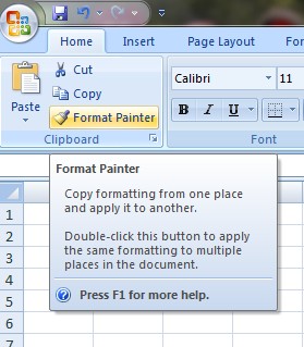
Here we can see that in cell A1 there is a text in bold, italic and underline format but the same text we can see in a different cell A3 but this is neither bold nor italic and underline, but if we take our cursor to cell A1 and click from mouse on the above shown Format Painter brush  icon and click on icon and paste the same to the cell i.e. A3 to change the format like the cell A1

It will be look like as follows that cell A3 has become same as cell A1 bold, italic and underlined.

Shortcut for above cell format like bold, italic and underline

Cntr B, for Bold, Cntr U for Underline and Cntr I for Italic

Simply Cntr B,U,I

So by this way we can use this tool to change format without going to format a cell option.


Thanks and good bye for now!


Narendra

Picking a Random Name from given list

Today we will discuss about random list i.e. how to look for a random name in the given excel list.

Here below we have a excel list from range A1:A14, and in range B2 there is value "Vimal" but the fact is cell B2 has a formula i.e. INDEX and RANDBETWEEN both formula has separate solution like Index has a list of names and randbetween has to pick any name from the give list so below is the example and we can understand in a very easy way.

Here in this example we are watching in this list A1:A14 it has 14 names so if we want  any name from this list, so put a randbetween formula, randbetween formula look for any no. value from the given range. And what index function does, it provides a list range as an array like range A1:A14

so simple index function provides a range and randbetween look for any no. value i.e. name from the list. So easily we can get the random no. or name from the given list.

Thanks

Narendra