Excel Data Validation

Excel Data Validation is a option in excel by which we  can restrict the operater by typing the false entry in the Excel sheet, it has some criteria for user and from this criteria or condition the user can not enter the wrong input.

We will understand this by following example:-

Go to Data Tab -->

Image 01

In this this image we can see that in the Data Tab --> Data Validation and when we click on Data Validation following image will appear

Image 02

In this 2nd image, there are three table ---> "Settings", "Input Message", "Error Alert" and then Validation criteria "Allow" :- Any Value

When we select a area in excel and apply this condition in data validation, this criteria accepts all the numbers or text, it does not have any restriction to the field. But when this feature will  restrict us to put incorrect data, we will learn in further in this  blog.

Now come to the second image :-

image 03

This is the all list of data validation :-

"Whole number", "Decimal", "List", "Date", "Time", "Text length", "Custom".

We  will discuss all of the above given option one by one.

"Input Message " is the second tab in the Data Validation box and the third one is "Error Alert"

Input Message box in Data Validation

Image 04

"Input Message" box display the message about the cell or area containing the validation about, like in the above image we can see that we  have a message like in "Title = => Serial No." and in the "Input message" box "Only put serial no. 1 to 10" and same we can see above in the excel coloured area, when we put our cursor into cell "C1" it displays the message as we put in the "Input message" box.

Error Alert box in Data Validation

See the image below :-

Image 05

Now in this Data Validation "Error Alert" message box,  we notice that we have checked the check box "Show error alert after invalid data is entered" if we do not check this check box then the message will not be displays.

Now come to "Style" and the option are "Stop", "Warning" and " Information" all the option are available for we that in which option we want to see the message from these three option.

Then "Title" is that what title we want to give that error message, we have put Wrong Input.

Then "Error Message" what message will pop up when someone will put wrong data in the validation field.

See the  below image :-

Image 06

We put "11" in the coloured field that field has validation and the message is showing that "Wrong Input" as the error title and message is "Please enter the no. between 1 to 10 only" this coloured area has validation to put data only from 1 to 10 not beyond this.

Criteria Examples of Data Validation

Any Value Data Validation

If we select this option in data validation that means we can put any data into the data validation field whether a numeric or a text one.

Whole Number Data Validation

Now come to second option Whole number, if we choose this option that means we can specify the maximum and minimum range in the validation area, see the image below :-

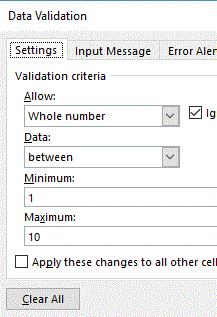
Image 07

We have set the limit between minimum "1"  and  maximum "10" the data validation field will accept the data with-in this range only not apart from that.

Decimal Data Validation

In this image we can see that we have set the data validation value  from 100 to 125 and this has a additional feature that it can accept the decimal figure also, like in the below image we can see "100.253" and "124.362" but not greater than "125". It accept the value in decimal also.

Image 08

List Data Validation

Now move forward to another option and it is "List" option in data validation. See the image below 

Image 09

In this image we can see that in cell "A1 to A3" we have put some name and now  the cursor position in cell "B1". In the "List" option in data validation, select "list" from allow field and type all the names in the "Source" field or drag the name range from "A1:A3", result would be same from both option and press "OK" then go to cell "B1" the following image will appear.

The drop down menu have been created by simple pressing "OK" button.

Image10

In the above image we can see that when we click on cell "B1" then a drop down menu list open with containing all the list details of from "A1 to A3".

Date Data Validation

In the below image the selected area has a data validation for the "date range". From start date contain the date range of cell "A1" and end date range contains the date of cell "B1".

Image 11

If any other date will be entered in the selected validated area the date will not be accepted by excel.

Time Data Validation

In the below image we have put the time range  in start time and end time and the selected area will not accept any time range apart from this time range.

Image 12

Text Length Data Validation

Text length validation option gives a condition that we can put the  text into a validation area, that we can only put the data according to the condition as shows in the below image.

Image 13

And if we try to write something beyond our validation condition  then it does not allow us to do that by showing below error message ,

Image 14

Custom Data Validation

Custom data validation is the validation when we put our own condition in the formula point and get the result as appear in the below image :-

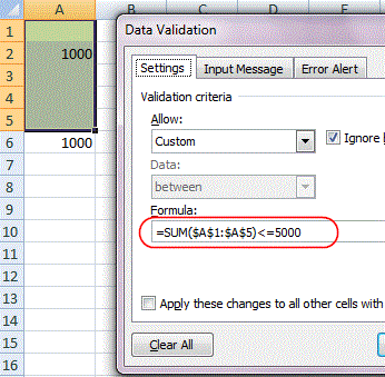
Image 15

And if we enter the value beyond  criteria then it shows the below message :-

Image 16

In this Custom Data Validation option we can create more formula's according to our need. 

Circle Invalid Data

If we have a data range and this data range contain a data validation of any given range as in the following image :- 

Image 17

In the above image we can see that we have given a range from 100 to 150, so the data range will accept the data from this criteria only but if there is any data beyond this range it will circle the cell, which is containing the the wrong value.

How to do that, just see below instruction and image :-

Excel Data - ->Data Validation --> Circle Invalid Data 

Image 18

and once you click on the "Circle Invalid Data" then the following result will come out from the selected data range which is containing the data validation.

Image 19

In this image we can see that which figure is beyond our data validation limit i.e. 100 to 150, the "Circle Invalid Data" option put a circle around that figure and again if we want to remove the circle then we have to follow this command. 

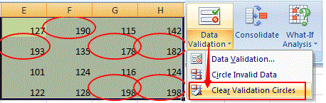
Go to Data -- ----  Data Validation ---- Clear Validation Circles and click on it.

Image 20

Once you click on the button "Circle Validation Circles" we will get the following image :-

Image 21

All the  red circles have been removed.

How to Remove Data Validation

Now we have learned all the option in data validation and now we will learn about how to remove data validation. Now simply follow the step 

Click Data ---- Data Validation ---- Click on Data Validation button and then click "Clear All" button, appearing below in the given image and then "OK" 

Image 22

All the data validation have been removed from the selected area and we can work on Excel as normally.

There is one more way to remove data validation from the given range. Simply go to a blank cell which does not contain any validation and copy it the go to the validation area and select all the validated area and right click as mentioned in the below image and clikc on  paste special.

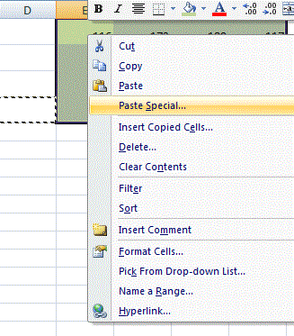
Image 23

Once you clik on paste special you will get the following image :-

Click on the "Validation" radio button and simply press "OK" and we are done.

This is very easy way to remove data validation from easy step.

Thanks and Regards

NarendrasExcelTips.blogspot.com

Excel Match Function

Match Function

In this tutorial we will learn about Match Function in Excel with some example and we will also learn a more about how this function works when we combine this function with Vlookup and Match.

Basically Match Function searches for a specified item in a range of cells and then returns the relative position of that item in the range.

So lets start with the following example:-

Image 01

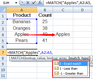
In this image we can see that this is a table which contain Column A "Product" and in Column B "Count" and in Column C there is a product name from the product list "Apples". The use of Match Function is to find the position of "Apples" in the list and in this list the position of "Apples"  is "3".

Now we will learn by break the argument of Match Function as follows :-

Syntax

MATCH(lookup_value, lookup_array, [match_type])

The MATCH function syntax has the following arguments:

lookup_value - The value to match in lookup_array.

lookup_array - The range of cells being searched.

match_type    -  Optional. The number -1, 0 or 1. The match_type argument specifies how Excel matches lookup_value with values in lookup_array. The default value for this argument is 1.


If Match_type is 1, [Match finds the largest value that is less than or equal to lookup_value and it requires sorting the lookup_array in ascending order, i.e. from small to large or from A to Z.]

If Match_type is 0, [Match finds the first value exactly equal to lookup_value  and lookup_array argument can be in any order.]

If match_type is -1 [Match finds the smallest value that is greater than or equal to lookup_value. The lookup_array must be sorted in descending order.]

1. Match returns the position of the matched value within lookup_array.
2. Match returns the #N/A error if no match is found.
3. Match is not case-sensitive.

If the lookup_array contains several occurrences of the lookup_value, the position of the first value will be returned.

We can understand this a little by the following example :-

Image 02

In the above image we put all three kind of formula (1,0,-1)

In the 1st formula, lookup_value is "35" but in the Column B there is no value appearing as "35", so in this formula we put match_type "1" because it will return a position of nearest and below of  value "35" and the position is 2nd, i.e. below "35", "34" is the nearest and below "35" value. So the  result is "2"

In the 2nd formula, lookup_value is "34" and Column B has the value "34" so we put match_type "0", and it gives us position of "34" is  2nd. So the result is "2".

In the 3rd formula, lookup_value is "52" and which exist in Column B but when we put  match_type (-1)  the result is  #N/A, The reason is #N/A is because as per the rule if the match_type "-1" then we have to sort the range in the form of descending order, so once we descending  the Column B then see what will be position of "52" 

Image 03

The position of "52" in count column in "1" and now we will learn formula combination with Match function.

Match Function with Vlookup

Following example is the best example to know that what is the use of Match Function with Vlookup.

Cell "G2" has a Vlookup formula which is showing in the  upper formula bar.

Here we can see that this is a simple Vlookup formula which returns a "Unit Price". Now we want to know that if we insert a new column between "Product Name" and "Unit Price" in this table, so will this effect to our result ?

Image 04

Lets understand in a new image :-

Now what we will do just insert a new column between Column A and Column B and see what will happen with the result "Unit Price" see the image below :-

Image 05

Here we can see that when we insert a new columns between Column A and Column B, the result of "Unit Price" have been change to "Exotic Liquids" form "19" as appearing in above "image 04" and which is not correct. So how to get the correct result.

Now in this situation "Match Function" comes in rescue.

Now we will combibe the the Match Function with Vlookup and then see what happened :-

Image 06

 

This image is the same as "image no 04" but in this image we get the result with the help of Vlookup and Match,  we can see the formula bar the formula is loaded by "Match Function". We have seen that there is no change in the result. It is same as we get by the single Vlookup.

Now we will do the same practical as we did in previous image to insert a new column bewtwee Column A and Column B and see what happen :-

Image 07

Now in this image we can see that we added a column "Supplier" between Column A and Column B. But after addition a new column we can see that there is no change on result, it is as before. So match function does not care about delete or add new column.

Now it is clear that the role of Match Function is to look for the matching figure and in this table Match Function search for Unit Price from the list A1:E1, and it does not matter that how many column we add or delete. The formula will produce the result accurately without any cell or column change or change in result.

Now this is clear that if Vlookup and Match function will work together, it will produce the dynamic result and one another benefit is that it prevents from error.

I hope this post has helped you understand how the Vlookup and Match function work together and produce a dynamic result.

Regards 

NarendrasExcelTips.Blogspot.com

Index Function

     Today we will learn about Index Function in Excel. Index Function in Excel is one of the most useful function. When we combine this function with another function like Match etc, it will produce the dynamic result.

The INDEX function returns a value or the reference to a value from within a table or range.

In the below image we can see the Index function has two different formula like :-

1.   Index (Array, Row_num,[Col_num]

2. Index (Reference, Row_num,[col_num],[area_num]

In the first formula it is Array and in the second function in place array it is Reference.

We will give separate example for both of the format.

Array form

We can see that some values are in the bracket like [column_num] and in second function [column_num] and [area_num].  i.e. if these values does not exist then we will consider these values as "0" and the function will produce the result by without these values.

Image 1

We will understand the use of Index Function in Excel by following example

Example 1.

Image 2

In the above image when we put the Index Formula such as:- = index(A2:E10,5,4)

In this example we can see the Index Function parameters like (Array, row_num, col_num)

Where  Array is                (A2:E10),

Row_num      is                     5

Col_num        is                     4

Simply the pure explanation is we want the result from area A2:E10, where Row_num is "5" and Col_num "4" and simply answer is "13". We can see red circled, the above image is the intersection of the Row_num and Col_num.

Example 2.

Image 3

In this example we can see the range is (A2:C11) where row_num is "6" and column_num is "3"

Result is from range (A2:C11),row_num(6),column_num(3)= "1943"

In range (A2:C11) intersection of row_num=6, and column_num=3 is "1943"

Example 3.

In the below given example, we can see that row_num and col_num  has the cell reference like:- "D2=Row_num" and "D3=Col_num"

Image 4

In this example if we change the "row_num" and "col_num" according to need then we do not need to change the formula, it will produce the result automatically, "Just try it" because in this example "row_num" and "col_num" are cell reference. So we can change the value.

Reference form

In the second part of Index Function, the first parameter is reference, which is supplied as a reference to one or more cell range. The syntax of reference is :

Index (reference, Row_num.[col_num],[area_num]

Where [col_num] and [area_num] is optional

See the following example to know it better :

Image 5

=INDEX((A2:C5,A7:C10),2,2,1)

In this image we can see that the whole range is divided in two section such as "A2:C5" and "A7:C10"  then come to "row_num" (2) and column_num(2) the and the last section is "area_num"

which is the important in this example. "Area_num" is telling to us that the figure we are looking for, is in which area, whether it is area_num =1 ("A2:C5")  or area_num =2 ("A7:C10")

In the above example if we put "2" in the area_num the result would be "Vaucheron & Constantin 18K" but if we put "1" in the area_num then result would be different i. e. "Cartier Tank 18K"

In our further tutorial we will learn to combine the Index Function with the other function like "Match", "Count" and will see that what kind of the result we will get.

Regards

NarendrasExcelTips.blogspot.com

How to Record a Macro in Excel

Recording a macro in Excel VBA is a very very useful tool. Why we use this tool to record a macro?

Reason is very simple that if we are doing the same task in Excel and again and again, then macro recorder comes in existence. We use macro recorder for reducing time taken in our daily task.

By the below given image we will understand macro recording step by step:-

Open the Excel and go to Developer tab and click on it.

                                                     Image 1

And then click on the Record Macro and following image will appear

                                Image 2

Once you click on the "OK" button in above image then macro will record everything, whatever action or step you will do in excel.

Main thing about macro recording is that it will record every single step, we will take. So my suggestion is plan first  to record macro and then record it and if you will not make a plan and start recording, it will record unnecessary step also.

Below is the details about above circled number in macro recorder box.

1. Macro Name

Macro name box where we can type the name of our macro, the first  character of macro must be a letter and macro name can not have a space like "My first macro", it should be "My_first_macro" and macro names are not case sensitive.

2.Assign Shortcut Key

In serial no. 2 we have to give a shortcut key for when we run the macro by key, we simply press the shortcut key and macro will run.

3. Store macro in

Third no. is store macro in, there is a drop down list. and we need to select the file from "Personal Macro Workbook, "New Workbook", and "This Workbook".

This Workbook.

Save the macro in the  current workbook, we are working with and macro will work on that file only.

New Workbook

Create macros that you can run in any new workbooks.

Personal Macro Workbook

We will choose this option if we want the run macro in every file we will work, it does not matter on whatever file we are working.

4. Description Box

In this box we will type the description about the macro that for what purpose the macro is created but this is optional not necessary.

Please the see the below of "Macro Recorder Box" image of figure entered.

                                                           Image 3

And now simply click on "OK"

Once you click "OK" then we will see that the record button will changes into "Stop
Recording" button, this means now Excel has started record our steps and when our step for macro recording is finished then we simply click on this "Stop Recording" button and macro is recorded successfully.

Simply I did something in excel for "Record a Macro" in below image :-

                                 Image 4


I type "a" in cell "C5" and "b" in cell "C7" and click on Stop Recording button, and see how a macro recorder record a macro in below image:-

                                        Image 5


First it type the Macro name " Sub Macro4 ()" and then record below mention thing like, first it select cell "C5" and then type "a" and then select cell "C7" and type "b" and then select cell "C8" and then I stop recording by pressing "Stop Recording Button" as appearing in the below image.

 

                                                               Image 6

And once we press stop recording button the macro recorder has finished its job, macro recording is done.

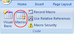
Now if we want to check our macro, simply go to Developer tab --> Macro and click on the "Macro" button

                                                                           Image 7

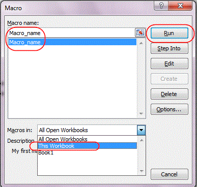
Once you click on the "Macro" button, the following image will appear

                                                                   Image 8

We will see that  macro name, we put "Macro_name" and below "Macro in"  means will work on the, the workbook we selected that time when we record the macro, select "This Workbook" and press "Run" button the will get the following image

                                                                          Image 9

Both the figure comes automatically in the cell "C5" and "C7" and another way to run this macro is simply type "Ctrl+Shift+L" because we have given a shortcut name to our macro. See Image 3.
And we will get the same result. try this...

This is the tutorial about "How to Record a Macro in Excel". and I will come soon about a new topic.

Regards

NarendrasExceltips.blogspot.com

Excel VBA Range Object

The Range Object in Excel VBA represents a single cell or multiple cells in excel worksheet and it is most important object of Excel VBA.

We can refer a single cell, multiple cells, a rows or a columns, a selection of cells. In this blog, we will give an overview of the properties and methods of Range Objects. Cells are the most important part of Excel and VBA and almost everything we do in Excel VBA start and end with cells.

There are several ways to referring a Range objects:-

1. Range property
2.  Cell property
3. Offset property
4. Union and Intersection Method
5. Current region
6. UsedRenge Property

Range Property

First we will study about what is a range property. Range property is cell or collection of cell and it depends totally as we write the VBA code. In the below given example we write the VBA code and execute it and see what happens, It will help us to understand Range property in a better way.

Next Code is

Next Code is

Next Code is

Next Code is

Cell Property

We can say that Excel is a Cells collection objects and there are multiple cells in a worksheet, so collection of cells is more complicated than collection of worksheet because cell comes in two dimensions.

A Cells  are a intersection of Rows and Columns, so in this case we have to mention two range, one of a row and second of a column like: - [ Cells(3,2).select], 3 for Rows i.e. Third Row, and 2 for Columns i.e. 2nd column. See the below example :-

Code No 1. 

We can see in see in the above image in the second row it is asking for the [Row Index] first and [Column Index] second. i.e. Row first and Column second.

Simply the intersection of Row 3 and Column 2, the value will be "3" as given in the coding.


Code No 2.

In the above image we can see that there are a different coding, Cells(1,2), Cells(4,2). First Cells(1,2) represents a cell which is intersection of First row and Second Column and second cells(4,2) represents a cell which intersection of Fourth row and second column i.e. the range will start from "B1:B4" and we can write this coding is "Range("B1:B4").value=3 Both the coding is correct and same.

But we are discussing about the Cell property, so we will choose the first one.

Offset Property

The Offset property provide another means for referring a range. Like a Cell property, Offset property takes two arguments, The first represents the number of Rows to offset and second represents number of Columns to offset.

The syntax for the Offset property is as follows:

Range.Offset(Row number to Offset, Column number to Offset)

Lets consider Range as A1 and Row no =1, Column no. = 3

Range("A1").Offset(Row Offset:=1, Column Offset:=3) or another way

Range("A1").Offset(1,3).value=11

See the image below :-

The quality of Offset property is,in the above coding Range("A1") is the starting point but when it enter the value it will not count "A1" it just leave that cell or range and count from next cell.

Simply in the  above example it will put the value cell "D2", as code explanation is after Range("A1"), first row and third column put the value "11"

Leave First row and First column as it starts from Range("A1") and then count row and column and enter the value.

Union and Intersection Property

Union and Intersection Method are another two method of range object, where Union method generate a range of two or more range. It can be understand by the below given image :-

Union Method

Here in this image we can see that, in the Excel sheet the shaded range is the combination of two ranges, [Range("A1:B3")] and [Range("B2:D4")]

So Union method range is the range of two or more ranges as we see in the above image and it can be the combination of more than two range also.

Intersect method

Intersect Method is just like the same as Union Method but in Union Method the range is  from two or more range but in Intersect Method represents the intersection of two ranges. We can understand this by below given image :-

Here in the above image we can understand that Intersect Method represents the intersection of two ranges. In this example we can see that intersection falls between two cells "B2" and "B3". We use Union and Intersect Method to find Union and Intersect between two or more ranges.

Current Region

Current Region is a range bounded by any combination of blank rows and blank columns.

We can understand the Current Region Property by the following image in a better way :-

In the above image we can see that every cell is connected with a new data containg cell, so when we apply Current Region property it select all the data which is connected by cell to cell but if any row or column is blank then the Current Region property will not include the range or data which is after blank row or column, as seen in the below image :-

Here we can see in the above example in the image, column is blank, the data has been deleted but column D contains some data and when we execute the code or command of Current Region it will select only two column which are connected by data cell to cell.

So when we apply Current Region Method to select  the range it will select only those cell which are connected with each other the Row and Column should not be blank otherwise the code will not consider the rest part of the data.

UsedRange Property

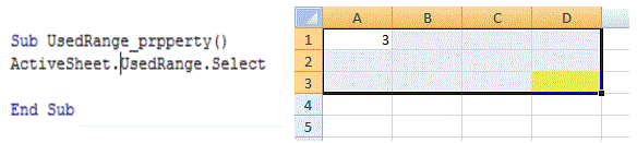
UsedRange Property is a worksheet property, it returns the are Range bounded by first used cell and last used cell.  "Used Cell" is defined as Cell contains formula, formatting, value that has ever been used or if the value now has been deleted also.

We will understand this by the below given image:-

In the above image we can see that there is no value after cell "A1" but the code is selecting all the cells up to "D3" because in the previous example cell "D3" has a value and deleted by later. 

So this is the quality of UsedRange property that it covers all the area from first cell to last cell contains data or formula or format, whether it has been deleted by later or still contains some data.

So in this tutorial we discuss the Excel VBA  Range Property Objects.

Please suggest for the improvement of this blog, your suggestion are welcome.

Regards

narendrasexceltips.blogspot.com